5k Pace and Race Time Predictor Examples

A 5k pace calculator helps translate a five-kilometre time into an average rate, while a race time predictor asks a different question about another distance. This set of worked examples keeps those tasks separate. We begin with exact distance-time relationships, then compare constant pace with an optional power-law scenario. All times are fictional arithmetic examples, not targets, fitness assessments or promises about what a particular runner will achieve.

Example one: five kilometres in thirty minutes

Thirty minutes contains 1,800 seconds. Divide by five kilometres to obtain 360 seconds per kilometre, displayed as 6:00/km. Multiply by 1.609344 to obtain 579.36384 seconds per mile, displayed as 9:39/mi. The speed equivalent is ten kilometres per hour, or approximately 6.2137 miles per hour. Each value describes the same entered average.

With kilometre splits selected, the cumulative rows are 6:00, 12:00, 18:00, 24:00 and 30:00. Each row covers a complete kilometre. A mile table would instead have three complete miles and a shorter final segment because five kilometres is approximately 3.1068559612 miles. The finish still corresponds to the entered thirty minutes, regardless of the split unit.

Use this example as a quick verification of the three modes. Pace mode takes five kilometres and thirty minutes. Time mode takes five kilometres and 6:00/km. Distance mode takes thirty minutes and 6:00/km. All three describe the same relationship. This consistency check is a useful way to notice a wrong unit or a value entered into an inactive field.

Example two: a twenty-five-minute 5k

Twenty-five minutes is 1,500 seconds, so dividing by five gives 300 seconds per kilometre: 5:00/km. The equivalent mile pace is 8:03/mi when rounded for display. Kilometre checkpoints occur at five, ten, fifteen, twenty and twenty-five minutes. Speed is twelve kilometres per hour. No prediction model is needed to obtain these values.

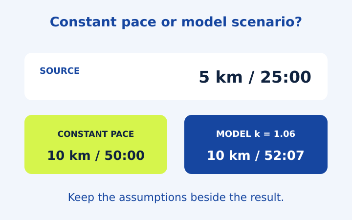
Now extend that exact average rate to ten kilometres as a hypothetical constant-pace exercise. Multiplying ten by five minutes gives fifty minutes. This operation answers what total time follows if the same average rate is maintained over twice the distance. It does not establish that the fictional source runner can maintain it. The assumption belongs in the sentence explaining the result.

That distinction matters when comparing this fifty-minute arithmetic with a power-law estimate. Different methods can return different values because they answer different questions. Rather than deciding one is wrong, identify what each holds constant. Constant pace keeps time per distance unchanged; a power law changes the modeled time-per-distance relationship through its exponent.

Example three: a partial final segment

Take a fictional 5.5-kilometre route completed at 6:00/km. In time mode, multiplication gives thirty-three minutes. The first five kilometre rows end at thirty minutes, and the final half-kilometre takes three minutes. The finishing row is a partial segment, so its duration is intentionally smaller than a full kilometre’s duration.

Switch the split unit to miles without altering distance or pace. The checkpoint locations and individual durations change, but the overall finish remains thirty-three minutes. The calculator computes those rows from the unrounded physical rate. It does not relabel kilometre row numbers as miles or use the displayed rounded mile pace as a new source input.

A note worth copying

Write route distance 5.5 km, assumed constant pace 6:00/km, finish scenario 33:00 and even splits. If the route was actually measured and timed, state that separately from the hypothetical assumption. A clear note tells the next reader whether the figures describe an observation, a planning exercise or a conversion. The same numbers can serve different purposes depending on those labels.

Example four: compare a power-law ten-kilometre scenario

The optional race-time model uses T2 = T1 × (D2/D1)^k. T1 is the source duration, D1 is its distance, D2 is the target distance and k is the selected exponent. The default exponent is 1.06. It is a fixed modeling choice that can be edited within the tool’s bounded range; the calculator does not estimate a personalized exponent from one activity.

Use the twenty-five-minute 5k as the source and ten kilometres as the target. The distance ratio is two, so the model gives 1,500 × 2^1.06 seconds, approximately 3,127.3973 seconds. Rounded to a clock display, that is 52:07. Constant pace gave 50:00, while the exponent above one produces a longer modeled time for the longer distance.

If the exponent is exactly one, the power law reduces to constant pace because the distance ratio is no longer raised above its linear relationship. A larger exponent increases the modeled cost of extending distance. Editing the exponent illustrates this mathematical sensitivity. It does not make the chosen value correct for an individual runner, and it should remain visible in any shared prediction note.

Example five: a half marathon target from the same source

Keep the twenty-five-minute source 5k and choose 21.0975 kilometres as the target. The ratio is 4.2195. With the default exponent of 1.06, the model yields approximately 6,900.299 seconds, displayed as 1:55:00 after whole-second rounding. The exact calculator output follows the unrounded ratio and exponent; do not derive it by multiplying a rounded ten-kilometre prediction.

At constant 5:00/km, the same target would instead take 6,329.25 seconds, displayed as 1:45:29. The gap reflects the different assumptions, not an additional measurement of the source runner. Neither result includes course profile, weather, interruptions, preparation or changes in performance. A single source distance and time cannot supply those missing details.

A primary study of recreational runners by Vickers and Vertosick examined race-time prediction and found limitations when a simple scaling formula was applied to marathon times. That context supports cautious labeling of a model output. It does not turn our editable exponent into a validated personal forecast or provide a training recommendation.

Compare scenarios without hiding their assumptions

When changing the target distance, retain the original source distance and duration. If you also change the source, the difference between outputs no longer isolates the target-distance effect. Similarly, changing both the exponent and the distance makes it harder to explain why a prediction moved. A useful worksheet changes one setting at a time and records the previous values for comparison.

Use the marathon and half marathon pace guide when your starting point is a chosen finishing-time scenario rather than another race result. Use the 5k pace and race-time calculator when you want to inspect the actual arithmetic behind either approach. Keep model estimates optional, clearly labeled and separate from recorded results.

The strongest conclusion from these examples is procedural: pair the correct distance and time, preserve units, read partial segments and identify the model being used. The calculator can make those relationships easier to see. Decisions about participation, preparation and personal goals require context beyond the fields on this page, and the generated note should never imply that such context has been evaluated.

Frequently asked questions

Put the numbers into your own note

Open the pace calculator with your own distance and time. Choose matching units, read the assumptions and copy the even-split note. Treat any race-time model as a scenario, not a promised performance.